语音增强性能评估相关函数（粉噪声、babble噪声、PESQ、STOI）

完成智能语音处理有关语音增强的实验后，发现周围同学找不到一些MATLAB有关的语音增强函数，为了可以方便后来人，我把我从GITHUB以及CSDN上“收罗”到的函数在这里进行分享，事不宜迟，请看下文！

给一段干净音频加粉红噪声

MATLAB官方工具箱中有一个关于音频的强大工具箱Audio Toolbox，里面自带了一个pinknoise的函数：

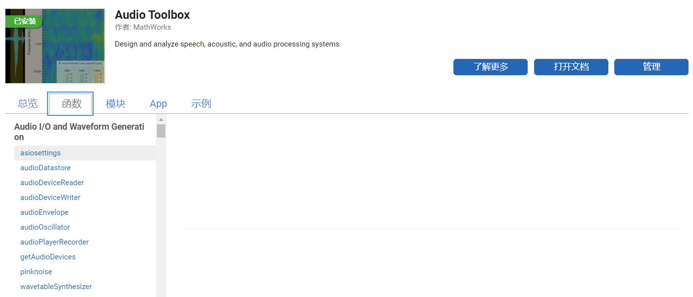
因此我们只要借助这个函数生成有关的加噪函数即可:

%音频加粉色噪声函数
function noisyMainStreet = add_pinknoise(audioIn,snr)
noise = pinknoise(size(audioIn),'like',audioIn);%借助matlab内置函数生成一个SNR未知的粉色噪声
noisePower = sum(noise.^2,1)/size(noise,1);%计算噪声能量
signalPower = sum(audioIn.^2,1)/size(audioIn,1);%计算音频能量
desiredSNR=snr;%期望设计信噪比
scaleFactor = sqrt(signalPower./(noisePower*(10^(desiredSNR/10))));%计算因子
noise = noise.*scaleFactor;%调整噪声能量
noisyMainStreet = noise + audioIn;%噪声合成
end

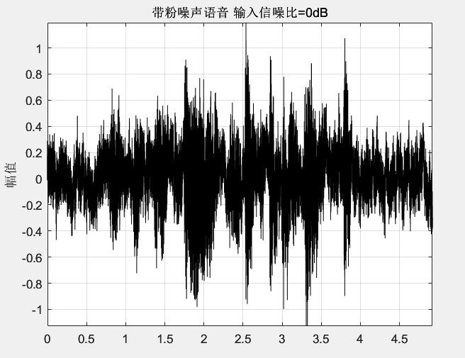
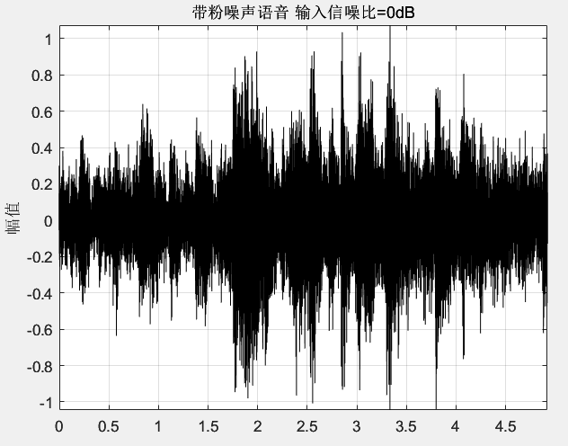
输入参数audioIn是不带噪声的原音频，输入参数snr是你期望加入噪声的信噪比，接下来展示如何使用这段函数:

[audio,fs]  = audioread("F1.wav");
audio = audio - mean(audio);%消除直流
audio = audio/max(abs(audio));%归一化
N = length(audio); %语音长度
time = (0:N-1)/fs;  %设计时间刻度

audio_withpinknoise = add_pinknoise(audio,0);
snr1 = round(SNR_singlech(audio,audio_withpinknoise));
disp(snr1)

plot(time,audio_withpinknoise,'k'); grid; axis tight;
title(['带粉噪声语音 输入信噪比=' num2str(snr1) 'dB']); ylabel('幅值')

结果如下所示:

给一段干净音频加babble噪声（背景多人人声）

借助上述生成粉噪相同的思路我们就能够生成babble噪声，但问题是系统并没有自带生成babble背景多人人声噪声，因此我们换个思路，把该带有该噪声的数字音频数据导入(load)进Matlab中

%音频加babble噪声函数
function noisyMainStreet = add_babblenoise(audioIn,fs,snr)
%导入babble文件
load babble.mat;
babble_fs = 19980;
babble_resamp_8k = resample(babble,fs,babble_fs);
desiredSNR=snr;%期望设计信噪比
Nx = length(audioIn);% 求出信号长
noise = babble_resamp_8k(1:Nx);   %截取babble噪声片段

noisePower = sum(noise.^2,1)/size(noise,1);%计算噪声能量
signalPower = sum(audioIn.^2,1)/size(audioIn,1);%计算音频能量
scaleFactor = sqrt(signalPower./(noisePower*(10^(desiredSNR/10))));%计算因子
noise = noise.*scaleFactor;%调整噪声能量
noisyMainStreet = noise + audioIn;%噪声合成
end

输入参数audioIn是不带噪声的原音频，输入参数snr是你期望加入噪声的信噪比，输入参数fs是原音频的频率，接下来展示如何使用这段函数:

[audio,fs]  = audioread("F1.wav");
audio = audio - mean(audio);%消除直流
audio = audio/max(abs(audio));%归一化
N = length(audio); %语音长度
time = (0:N-1)/fs;  %设计时间刻度

audio_withbabblenoise = add_babblenoise(audio,fs,0);
snr1 = SNR_singlech(audio,audio_withbabblenoise);
disp(snr1)

plot(time,audio_withbabblenoise,'k'); grid; axis tight;
title(['带粉噪声语音 输入信噪比=' num2str(snr1) 'dB']); ylabel('幅值')

结果如下所示:

STOI函数

STOI(短时语音可懂度),这部分代码也是借助GITHUB链接:
STOI函数

function d = STOI(x, y, fs_signal)
%   d = stoi(x, y, fs_signal) returns the output of the short-time
%   objective intelligibility (STOI) measure described in [1, 2], where x 
%   and y denote the clean and processed speech, respectively, with sample
%   rate fs_signal in Hz. The output d is expected to have a monotonic 
%   relation with the subjective speech-intelligibility, where a higher d 
%   denotes better intelligible speech. See [1, 2] for more details.
%
%   References:
%      [1] C.H.Taal, R.C.Hendriks, R.Heusdens, J.Jensen 'A Short-Time
%      Objective Intelligibility Measure for Time-Frequency Weighted Noisy
%      Speech', ICASSP 2010, Texas, Dallas.
%
%      [2] C.H.Taal, R.C.Hendriks, R.Heusdens, J.Jensen 'An Algorithm for 
%      Intelligibility Prediction of Time-Frequency Weighted Noisy Speech', 
%      IEEE Transactions on Audio, Speech, and Language Processing, 2011. 
%
%
% Copyright 2009: Delft University of Technology, Signal & Information
% Processing Lab. The software is free for non-commercial use. This program
% comes WITHOUT ANY WARRANTY.
%
%
%
% Updates:
% 2011-04-26 Using the more efficient 'taa_corr' instead of 'corr'

if length(x)~=length(y)
    error('x and y should have the same length');
end

% initialization
x           = x(:);                             % clean speech column vector
y           = y(:);                             % processed speech column vector

fs          = 10000;                            % sample rate of proposed intelligibility measure
N_frame    	= 256;                              % window support
K           = 512;                              % FFT size
J           = 15;                               % Number of 1/3 octave bands
mn          = 150;                              % Center frequency of first 1/3 octave band in Hz.
H           = thirdoct(fs, K, J, mn);           % Get 1/3 octave band matrix
N           = 30;                               % Number of frames for intermediate intelligibility measure (Length analysis window)
Beta        = -15;                           	% lower SDR-bound
dyn_range   = 40;                               % speech dynamic range

% resample signals if other samplerate is used than fs
if fs_signal ~= fs
    x	= resample(x, fs, fs_signal);
    y 	= resample(y, fs, fs_signal);
end

% remove silent frames
[x y] = removeSilentFrames(x, y, dyn_range, N_frame, N_frame/2);

% apply 1/3 octave band TF-decomposition
x_hat     	= stdft(x, N_frame, N_frame/2, K); 	% apply short-time DFT to clean speech
y_hat     	= stdft(y, N_frame, N_frame/2, K); 	% apply short-time DFT to processed speech

x_hat       = x_hat(:, 1:(K/2+1)).';         	% take clean single-sided spectrum
y_hat       = y_hat(:, 1:(K/2+1)).';        	% take processed single-sided spectrum

X           = zeros(J, size(x_hat, 2));         % init memory for clean speech 1/3 octave band TF-representation 
Y           = zeros(J, size(y_hat, 2));         % init memory for processed speech 1/3 octave band TF-representation 

for i = 1:size(x_hat, 2)
    X(:, i)	= sqrt(H*abs(x_hat(:, i)).^2);      % apply 1/3 octave bands as described in Eq.(1) [1]
    Y(:, i)	= sqrt(H*abs(y_hat(:, i)).^2);
end

% loop al segments of length N and obtain intermediate intelligibility measure for all TF-regions
d_interm  	= zeros(J, length(N:size(X, 2)));                               % init memory for intermediate intelligibility measure
c           = 10^(-Beta/20);                                                % constant for clipping procedure

for m = N:size(X, 2)
    X_seg  	= X(:, (m-N+1):m);                                              % region with length N of clean TF-units for all j
    Y_seg  	= Y(:, (m-N+1):m);                                              % region with length N of processed TF-units for all j
    alpha   = sqrt(sum(X_seg.^2, 2)./sum(Y_seg.^2, 2));                     % obtain scale factor for normalizing processed TF-region for all j
    aY_seg 	= Y_seg.*repmat(alpha, [1 N]);                               	% obtain \alpha*Y_j(n) from Eq.(2) [1]
    for j = 1:J
      	Y_prime             = min(aY_seg(j, :), X_seg(j, :)+X_seg(j, :)*c); % apply clipping from Eq.(3)   	
        d_interm(j, m-N+1)  = taa_corr(X_seg(j, :).', Y_prime(:));          % obtain correlation coeffecient from Eq.(4) [1]
    end
end
        
d = mean(d_interm(:));                                                      % combine all intermediate intelligibility measures as in Eq.(4) [1]

%%
function  [A cf] = thirdoct(fs, N_fft, numBands, mn)
%   [A CF] = THIRDOCT(FS, N_FFT, NUMBANDS, MN) returns 1/3 octave band matrix
%   inputs:
%       FS:         samplerate 
%       N_FFT:      FFT size
%       NUMBANDS:   number of bands
%       MN:         center frequency of first 1/3 octave band
%   outputs:
%       A:          octave band matrix
%       CF:         center frequencies

f               = linspace(0, fs, N_fft+1);
f               = f(1:(N_fft/2+1));
k               = 0:(numBands-1); 
cf              = 2.^(k/3)*mn;
fl              = sqrt((2.^(k/3)*mn).*2.^((k-1)/3)*mn);
fr              = sqrt((2.^(k/3)*mn).*2.^((k+1)/3)*mn);
A               = zeros(numBands, length(f));

for i = 1:(length(cf))
    [a b]                   = min((f-fl(i)).^2);
    fl(i)                   = f(b);
    fl_ii                   = b;

	[a b]                   = min((f-fr(i)).^2);
    fr(i)                   = f(b);
    fr_ii                   = b;
    A(i,fl_ii:(fr_ii-1))	= 1;
end

rnk         = sum(A, 2);
numBands  	= find((rnk(2:end)>=rnk(1:(end-1))) & (rnk(2:end)~=0)~=0, 1, 'last' )+1;
A           = A(1:numBands, :);
cf          = cf(1:numBands);

%%
function x_stdft = stdft(x, N, K, N_fft)
%   X_STDFT = X_STDFT(X, N, K, N_FFT) returns the short-time
%	hanning-windowed dft of X with frame-size N, overlap K and DFT size
%   N_FFT. The columns and rows of X_STDFT denote the frame-index and
%   dft-bin index, respectively.

frames      = 1:K:(length(x)-N);
x_stdft     = zeros(length(frames), N_fft);

w           = hanning(N);
x           = x(:);

for i = 1:length(frames)
    ii              = frames(i):(frames(i)+N-1);
	x_stdft(i, :) 	= fft(x(ii).*w, N_fft);
end

%%
function [x_sil y_sil] = removeSilentFrames(x, y, range, N, K)
%   [X_SIL Y_SIL] = REMOVESILENTFRAMES(X, Y, RANGE, N, K) X and Y
%   are segmented with frame-length N and overlap K, where the maximum energy
%   of all frames of X is determined, say X_MAX. X_SIL and Y_SIL are the
%   reconstructed signals, excluding the frames, where the energy of a frame
%   of X is smaller than X_MAX-RANGE

x       = x(:);
y       = y(:);

frames  = 1:K:(length(x)-N);
w       = hanning(N);
msk     = zeros(size(frames));

for j = 1:length(frames)
    jj      = frames(j):(frames(j)+N-1);
    msk(j) 	= 20*log10(norm(x(jj).*w)./sqrt(N));
end

msk     = (msk-max(msk)+range)>0;
count   = 1;

x_sil   = zeros(size(x));
y_sil   = zeros(size(y));

for j = 1:length(frames)
    if msk(j)
        jj_i            = frames(j):(frames(j)+N-1);
        jj_o            = frames(count):(frames(count)+N-1);
        x_sil(jj_o)     = x_sil(jj_o) + x(jj_i).*w;
        y_sil(jj_o)  	= y_sil(jj_o) + y(jj_i).*w;
        count           = count+1;
    end
end

x_sil = x_sil(1:jj_o(end));
y_sil = y_sil(1:jj_o(end));

%%
function rho = taa_corr(x, y)
%   RHO = TAA_CORR(X, Y) Returns correlation coeffecient between column
%   vectors x and y. Gives same results as 'corr' from statistics toolbox.
xn    	= x-mean(x);
xn  	= xn/sqrt(sum(xn.^2));
yn   	= y-mean(y);
yn    	= yn/sqrt(sum(yn.^2));
rho   	= sum(xn.*yn);

PESQ函数

由于给出的PESQ代码过于长，在这里粘贴影响篇幅，因此给出GITHUB链接，读者自行前往链接复制粘贴。

PESQ函数

(新手第一次写博客，如有错误和不好的地方，请多担待，另外对程序有问题请提出噢！)